§ 1.2 Module 1 — When Voice Became Data
Sound into Numbers: Sampling, PCM, and G.711
If a function contains no frequencies higher than W, it is completely determined by giving its ordinates at a series of points spaced 1/2W seconds apart.— Claude Shannon, “Communication in the Presence of Noise,” 1949
By the end of this lesson
- Apply the sampling theorem: predict alias frequencies and choose valid sample rates
- Implement quantization and verify the ~6 dB-per-bit SNR rule
- Explain μ-law/A-law companding and why G.711 companded
- Explain why WebRTC standardizes on 48 kHz internally (Nyquist headroom, not superhuman hearing)
Historical note
Digital voice was invented twice: once on paper, once in copper. In 1938 Alec Reeves, a British engineer at ITT’s Paris laboratory, patented pulse-code modulation — represent a waveform as a stream of numbered pulses — a decade before any electronics could afford to do it. The theory caught up in stages: Harry Nyquist’s 1928 Bell System Technical Journal paper “Certain Topics in Telegraph Transmission Theory” bounded how many pulses a channel could carry; Claude Shannon proved the sampling theorem in 1949; and in 1948 Bernard Oliver, John Pierce, and Shannon published “The Philosophy of PCM,” arguing that digits, unlike analog voltages, could be regenerated perfectly at every repeater. The copper arrived in 1962, when Illinois Bell put the first T1 carrier into service between Chicago-area central offices: 24 telephone channels, each sampled 8,000 times per second at 8 bits, multiplexed onto two ordinary wire pairs at 1.544 Mbit/s. The CCITT froze that per-channel format in 1972 as Recommendation G.711. Every number in this lesson — 8 kHz, 8 bits, 64 kbit/s — was fixed by that 1962 arithmetic, and it still sets the sound of “telephone quality” inside every WebRTC call that touches the phone network.
1.2.1The sampling theorem, and what aliasing punishes
An analog microphone signal is a continuously varying voltage. To digitize it, a sampler measures that voltage at strictly regular intervals — the sample rate fs, in samples per second. The counterintuitive claim, the one Reeves’s contemporaries doubted, is that nothing is lost: Shannon’s sampling theorem says a signal containing no energy above some bandwidth B is exactly recoverable from its samples, provided fs > 2B. Twice the highest frequency is not a rule of thumb; it is a mathematical boundary, and the frequency fs/2 is called the Nyquist frequency in honor of the 1928 result.
The boundary is enforced by a specific failure mode. A sampler cannot tell a tone at frequency f from a tone at f + fs, or from fs − f: their sample values are identical. Any input energy above the Nyquist frequency is therefore folded back into the band below it, masquerading as a lower frequency. This is aliasing, and it is not distortion in the forgiving, analog sense — it is a new, unrelated tone sitting where no tone was played. The alias of a tone at f is found by reducing f modulo fs, then reflecting anything above fs/2 down to fs − f. Sample a 5 kHz whistle at 8,000 Hz and your listener hears 3 kHz; sample 9 kHz and they hear 1 kHz. Figure 1.2 shows the trap: the samples of the 5 kHz input lie perfectly on a 3 kHz sinusoid, and no algorithm downstream can ever know which one was played.
Because folding is irreversible, every practical digitizer places an analog low-pass anti-aliasing filter before the sampler, discarding energy above Nyquist while it is still merely inaudible rather than destructive. This is also where the phone network’s numbers come from. Bell engineers had long band-limited speech channels to roughly 300–3,400 Hz — intelligible, if thin. A 4 kHz channel allocation, doubled per Nyquist, gives 8,000 samples per second, with the 3,400–4,000 Hz gap left as transition room so a realizable analog filter could roll off in time. The sample rate of every telephone call since 1962 is, quite literally, a filter specification with margin.
1.2.2Quantization: the price of each bit
Sampling makes time discrete; quantization makes amplitude discrete, and unlike sampling it genuinely destroys information. A b-bit quantizer rounds each sample to the nearest of 2b levels spread across the converter’s full scale. The rounding residue behaves, for busy signals, like an added noise floor: uniformly distributed within ±half a step, with power step²/12. Work through the algebra for a full-scale sine wave and a b-bit quantizer, and the signal-to-noise ratio comes out to
SNR = 6.02·b + 1.76 dB (full-scale sinusoid, uniform quantizer)Listing 1.1 — The 6 dB-per-bit rule. Each added bit doubles the level count, halves the step, and buys 20·log₁₀(2) ≈ 6.02 dB.
Amplitudes in digital audio are measured against the converter’s ceiling in dBFS — decibels relative to full scale, where 0 dBFS is the largest representable value and everything real is negative. The 6 dB/bit rule then reads directly as dynamic range: 16-bit audio (CD, and the Int16 samples you will meet in Web Audio worklets) offers about 98 dB between full scale and the noise floor; 8-bit linear offers about 50 dB. Fifty decibels sounds adequate until you remember that the rule was derived for a full-scale signal. Quantization noise is a fixed floor: a quiet talker at −40 dBFS on an 8-bit linear channel enjoys not 50 dB of SNR but roughly 10 — audibly gritty, like sand poured over the whisper. Speech routinely swings 40 dB between a raised voice and trailing consonants, before you add the variation between loud and faint telephone lines.
So the 1962 designers faced an ugly trade. Twelve or thirteen linear bits would cover speech comfortably — but T1’s budget was 8 bits per sample, because 24 channels × 8,000 Hz × 8 bits had to fit the 1.544 Mbit/s the copper could carry. The escape was to make the steps unequal.
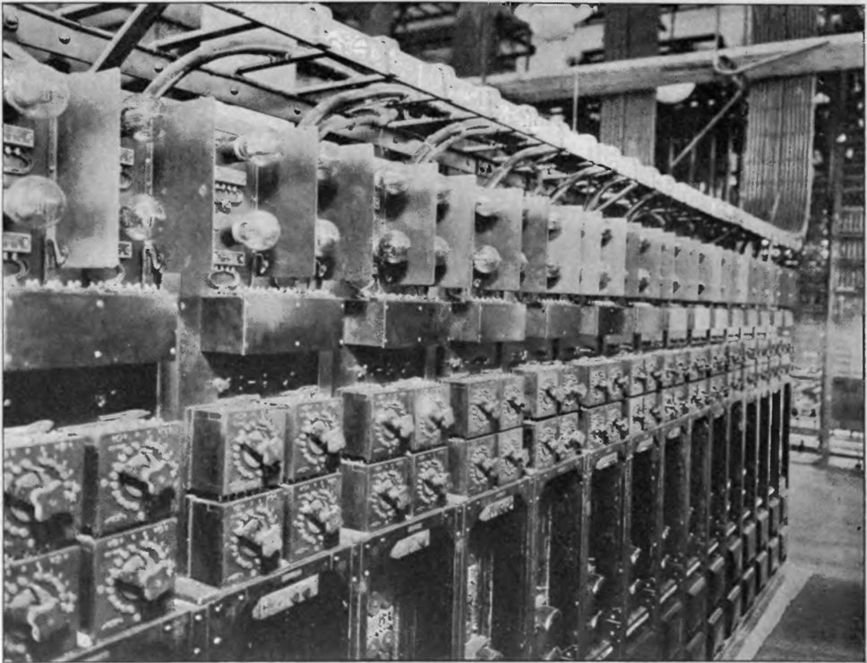
Early Audion repeaters. Amplifying an analogue signal also amplifies its accumulated noise, and the degradation compounds with every hop — the problem digital encoding was invented to escape, because a regenerated sample either arrives correct or does not arrive.
Bancroft GherardiPublic domainWikimedia Commons
Interactive lab bench
The sampler and the fold — 8 kHz is a filter specification
A 3D instrument you drive yourself, one variable at a time. It needs JavaScript and WebGL, so it is not shown in this static copy of the page.
new AudioContext({ sampleRate: 16000 }) is honoured by Chrome and Firefox but was long ignored or thrown on by Safari, and it has no effect on the capture rate anyway — WebRTC resamples internally. On macOS the hardware may run at 44,100 Hz while the getUserMedia track reports 48,000. On many Android devices the capture path is locked to 16 kHz when echoCancellation: true selects the hardware AEC, so your "fullband Opus" call is upsampled narrowband and no stat tells you.
Read audioContext.sampleRate after construction and never hard-code 48000 in your DSP. On Chrome, track.getSettings().sampleRate reveals the actual capture rate; if it reads 16000 on Android and you need wideband, try echoCancellation: false and accept that you now own echo control.
1.2.3Companding: G.711’s logarithmic bargain
The insight is perceptual as much as mathematical: hearing judges loudness ratios, not differences, so quantization error matters relative to the signal carrying it. A quantizer with fine steps near zero and coarse steps near full scale spreads a roughly constant signal-to-noise ratio across the whole dynamic range — compressing on encode and expanding on decode, hence companding. G.711, standardized by the CCITT in 1972, defines two logarithmic curves: μ-law (μ = 255), deployed in North America and Japan, and A-law (A = 87.6), deployed in Europe and most elsewhere; international trunks convert on the μ-law side. Both compress each sample into 8 bits: one sign bit, three bits selecting one of eight exponentially sized segments, and four bits placing the sample linearly within its segment — a piecewise-linear, hardware-friendly approximation of a logarithm.
// G.711 mu-law, the 1972 algorithm in JavaScript
const BIAS = 0x84;                       // 132
const SEG_END = [0xFF, 0x1FF, 0x3FF, 0x7FF,
                 0xFFF, 0x1FFF, 0x3FFF, 0x7FFF];

function muLawEncode(sample) {           // Int16 -> byte
  const mask = sample < 0 ? 0x7F : 0xFF;
  let mag = Math.min(Math.abs(sample), 32635) + BIAS;
  let seg = 0;
  while (seg < 8 && mag > SEG_END[seg]) seg++;
  return ((seg << 4) | ((mag >> (seg + 3)) & 0x0F)) ^ mask;
}
Listing 1.2 — μ-law encoding: sign, segment, mantissa, inversion. Eight bits that behave like fourteen.
The bargain pays off exactly where linear 8-bit fails. For small signals, 8-bit μ-law performs like roughly 14-bit linear PCM (A-law like 13-bit), holding SNR near 38 dB across some 40 dB of input level instead of letting it collapse with the signal. The cost is a slightly noisier ceiling at full scale — a trade speech accepts gladly. The resulting stream, 8,000 samples × 8 bits = 64 kbit/s, is the DS0, the indivisible unit around which the entire digital telephone hierarchy — T1, E1, ISDN, SS7 trunking — was sized. And it never left: G.711’s two flavors survive inside WebRTC as the static RTP payload types 0 (PCMU) and 8 (PCMA), and RFC 7874 makes G.711 — alongside Opus — mandatory for every WebRTC endpoint, precisely so the browser can always meet a 1972 telephone gateway on its own terms.
1.2.4The sample-rate zoo, and why WebRTC settled on 48 kHz
Telephony’s 8 kHz was only the first entry in a menagerie of rates, each an artifact of the medium that bore it. 16 kHz — “wideband,” a 7 kHz audio band — arrived with ITU-T G.722 in 1988 and was marketed decades later as HD Voice. 44.1 kHz is a videotape number: Sony and Philips fixed it in the 1980 Compact Disc Red Book because early digital masters were stored on video recorders, and three samples per video line worked out to exactly 44,100 per second on both NTSC and PAL machines. 48 kHz is the professional and broadcast rate — adopted by the AES, used by DAT recorders from 1987 — chosen for clean arithmetic against film and video frame rates and generous anti-alias filter margins. Modern audio hardware descends from that lineage: virtually every laptop and phone codec chip clocks natively at 48 kHz.
WebRTC standardized on the last of these. Opus (RFC 6716, 2012 — Jean-Marc Valin, Koen Vos, and Timothy Terriberry, fusing Skype’s SILK with Xiph.Org’s CELT) is a 48 kHz codec: whatever bandwidth it actually encodes, its RTP timestamps always tick at 48 kHz (RFC 7587), and its full-band mode covers everything human hearing can use. libwebrtc’s voice pipeline — echo cancellation, noise suppression, gain control — likewise runs at a common internal rate of 48 kHz, resampling whatever the microphone delivers through getUserMedia (often 44.1 kHz on consumer hardware) on the way in. When your WebRTC call sounds present and close while the circuit-switched leg patched in from a conference bridge sounds distant and thin, you are hearing sixty years of sampling decisions side by side: sibilants and consonant edges live above 3.4 kHz, and G.711’s anti-alias filter removed them in the name of 1962’s copper budget.
A common error
“WebRTC uses 48 kHz because it can carry sound up to 48 kHz” — or because engineers believed anyone could hear that high. Neither. Human hearing tops out near 20 kHz and retreats with age; Nyquist says 48 kHz sampling captures everything below 24 kHz. The extra 4 kHz above audibility is filter headroom — an anti-aliasing filter can roll off gently between 20 and 24 kHz instead of falling off a cliff — and the rest is convention: 48 kHz is what professional audio, film, and (consequently) commodity hardware clocks already speak. The rate was chosen to make engineering easy, not hearing superhuman.
The through-line of this lesson is worth stating plainly: every sample rate is a bandwidth claim, and every bit depth is a noise-floor claim. 8 kHz/8-bit companded says “intelligible speech, telephone budget, 1962.” 48 kHz says “all of human hearing, with room for the filters, 2012.” In the next lesson these samples meet the packet network — and the timing guarantees the circuit gave them for free disappear.
Build the two halves of 1962 yourself: a sampler-quantizer that lets you measure the 6 dB/bit rule and predict aliases, then the actual G.711 μ-law compander, graded byte-for-byte against the reference tables.
Lab 1
Build a Quantizer, Hear the Alias
Graded in the browser against 4 assertions; the editor and harness require JavaScript.
Lab 2
Implement the μ-law Compander
Graded in the browser against 4 assertions; the editor and harness require JavaScript.
Check your understanding
Auto-graded check
4 auto-graded questions with an explanation for every wrong answer. Requires JavaScript. (m1-l2-quiz)
Interactive lab bench
Companding — 256 levels, and where you put them
A 3D instrument you drive yourself, one variable at a time. It needs JavaScript and WebGL, so it is not shown in this static copy of the page.
¶Field quirks
What the specifications say, and what the browsers actually do, are two different documents. These are the divergences that cost production teams their weekends.
Web Audio and AudioWorklet hand you Float32Array nominally in [-1, 1], but nothing clamps it: a gain node, a sum of sources, or an over-driven mic will hand you 1.4. The textbook conversion Math.round(x * 32767) then overflows the int16 range, and if you write into an Int16Array the value wraps from +32767 to a large negative number. The audible result is a loud click on every peak, which sounds exactly like a network glitch and gets debugged as one for days.
Clamp before scaling: Math.max(-1, Math.min(1, x)), then multiply by 32767 for positives and 32768 for negatives (the range is asymmetric). If you are round-tripping to int16 and back, expect to see a noise floor around -90 dBFS; that is quantisation, not a bug.
G.711 appears in WebRTC as PCMU (payload type 0) and PCMA (payload type 8) — static assignments from RFC 3551, still negotiated because PSTN gateways want them. Their RTP clock rate is 8000, so a 20 ms frame advances the timestamp by 160, not by 960 as Opus does at 48 kHz. Any code that converts RTP timestamps to wall time with a hard-coded divisor produces a 6x error the moment a call falls back to G.711, and the fallback happens silently when a gateway is in the path.
Always read the clock rate from the negotiated codec: getStats() exposes it as RTCCodecStats.clockRate, joined via inbound-rtp.codecId. Note that video is always 90000 regardless of frame rate, and Opus always declares 48000 regardless of the actual audio bandwidth.
A 20 ms G.711 frame is 160 bytes of payload. Add 12 bytes of RTP header, 8 of UDP, 20 of IPv4, and a 10-byte SRTP authentication tag and you are sending 210 bytes 50 times per second — 84 kbit/s, or roughly 96 kbit/s over a TURN relay with the ChannelData framing and Ethernet headers. Capacity plans built from codec bitrates under-provision by 30–50 % for audio, and the error is worst exactly where bandwidth is scarce.
Plan from wire bitrate, and in getStats() remember that bytesSent is payload only — headerBytesSent is a separate counter you must add. The transport stats object gives you the honest figure including STUN, DTLS, and RTCP.
The Impossible Call: WebRTC from First Principles to Production · Module 1, Lesson 2